Exponential VS Logarithms
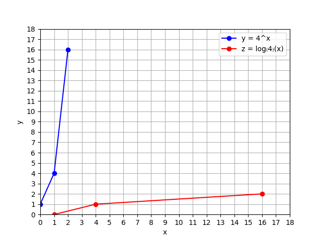
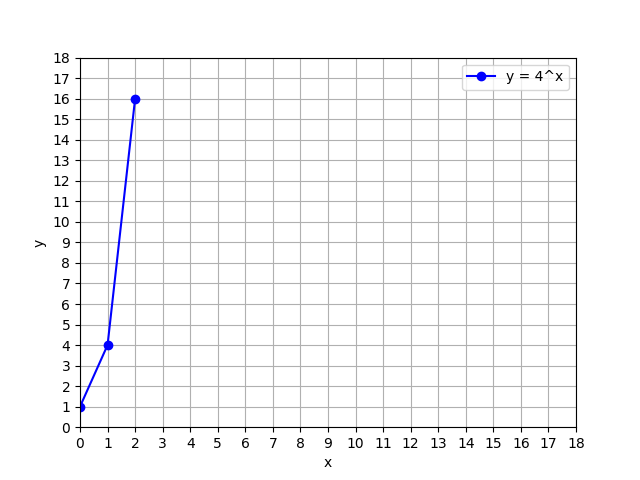
The 3 points plotted below are on the graph of \(y=b^x\) for \(b=4\).
\[\begin{array}{c|c} x & y = b^x \\ \hline 0 & 1 \\ 1 & 4 \\ 2 & 16 \\ \end{array}\]
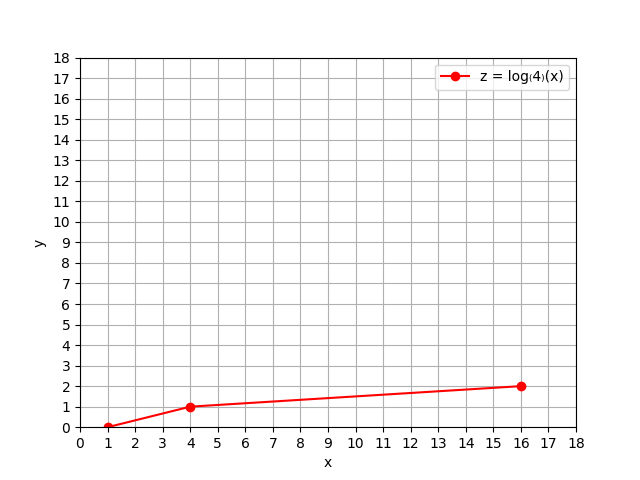
Based only on these 3 points, we plot the 3 corresponding points that must be on the graph of \(y=\log_{b}(x)\).
\[\begin{array}{c|c} x & y=\log_b(x) \\ \hline 1 & \log_b(1)=0 \\ 4 & \log_b(4)=1 \\ 16 & \log_b(16)=2 \\ \end{array}\]
And the whole reason is to give you this appreciation that these are inverse functions of each other.
The Python code
import matplotlib.pyplot as plt
import sympy as sp

def create_plot(from_tick, to_tick):
    # Create an empty plot
    plt.figure()

    # Set the x and y-axis limits
    plt.xlim(from_tick, to_tick)
    plt.ylim(from_tick, to_tick)

    # Define ticks for both axes
    ticks = list(range(from_tick, to_tick + 1))  # Include toTick in ticks

    # Set the x and y-axis ticks
    plt.xticks(ticks)
    plt.yticks(ticks)


def f_exponential(b, x):
    # Define y = b**x and plot it at x = 0,1,2
    y = b ** x
    x_vals = [0, 1, 2]
    y_vals = [float(y.subs(x, val)) for val in x_vals]
    plt.plot(
        x_vals,
        y_vals,
        marker='o',  # straight quotes, no extra spaces
        linestyle='-',
        color='b',
        label=f'y = {b}^x'
    )


def f_logarithms(b):
    # Define z = log base b of x
    y = sp.log(x, b)
    x_values = [1, 4, 16]
    y_values = [y.subs(x, val) for val in x_values]
    y_values = [float(val) for val in y_values]
    plt.plot(
        x_values,
        y_values,
        marker='o',
        linestyle='-',
        color='r',
        label=f'z = log₍{b}₎(x)'
    )


def show_plot():
    plt.xlabel('x')
    plt.ylabel('y')
    plt.grid(True)
    plt.legend()
    plt.show()


# --- Main code ---
b = 4
x = sp.symbols('x')

create_plot(0, 18)

# actually draw the curve
f_exponential(b, x)

f_logarithms(b)
# then label and display
show_plot()